All About Rooflines

Source: All About Rooflines, part of How To Scale Your Model, published 2025-02-04.

This is a Korean lecture-note adaptation, not a line-by-line full translation. The goal is to explain the roofline model and connect it to the inference measurements in this repository.

Selected figures from the JAX Scaling Book are reused under the repository’s MIT License. Additional SVG diagrams are redrawn locally in this repository’s editorial diagram style.

Reading Map

이 글은 TPU/GPU/DSA 글을 읽기 전에 필요한 성능 모델을 정리한다.

핵심 질문은 다음이다.

어떤 연산이 왜 5ms가 아니라 50ms 걸리는가?

답은 보통 세 가지 상한에 의해 결정된다.

Constraint	Unit	Meaning
Compute throughput	FLOPs/s or OPs/s	연산기가 초당 처리할 수 있는 연산량
Memory / network bandwidth	bytes/s	데이터를 이동할 수 있는 속도
Memory capacity	bytes	데이터가 물리적으로 들어갈 수 있는 크기

Roofline model은 이 중 compute throughput과 bandwidth를 함께 써서 어떤 workload가 compute-bound인지 memory-bound인지 빠르게 판단하는 방법이다.

이 그림에서 x축은 arithmetic intensity, y축은 달성 가능한 처리량이다. 왼쪽 사선 구간에서는 bandwidth가 성능을 제한한다. 오른쪽 수평 구간에서는 compute peak가 성능을 제한한다.

원문은 같은 아이디어를 log-log plot과 여러 bandwidth line으로도 보여준다.

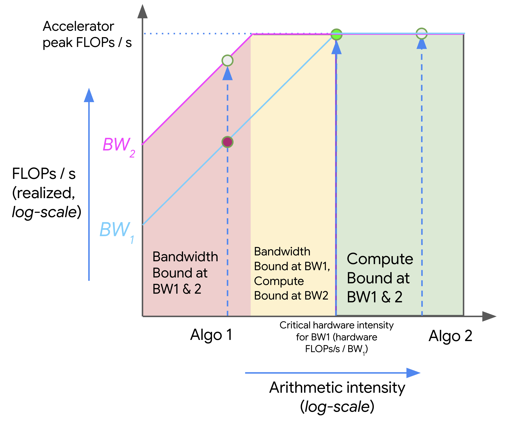
Source: JAX Scaling Book, “All About Rooflines”, MIT License. The original figure shows how algorithms with different arithmetic intensities move between bandwidth-bound and compute-bound regions as available bandwidth changes.

1. 시간은 어디에서 쓰이는가?

가장 먼저 계산해야 하는 것은 두 시간이다.

T_math = Computation FLOPs / Accelerator FLOPs/s

T_comms = Communication Bytes / Bandwidth Bytes/s

여기서 communication은 반드시 network만 뜻하지 않는다. HBM에서 Tensor Core로 값을 읽는 것도 communication이고, GPU 사이에 activation을 보내는 것도 communication이다.

Case	Communication meaning
Single GPU matmul	HBM -> SM/Tensor Core data movement
TPU matmul	HBM -> VMEM -> MXU data movement
Tensor parallelism	GPU/TPU 사이 activation collective
MoE expert parallelism	token AllToAll
CPU offload	host memory / PCIe / network path

실제 runtime은 compute와 communication을 얼마나 overlap할 수 있는지에 따라 달라진다.

Lower bound = max(T_math, T_comms)
Upper bound = T_math + T_comms

완전히 overlap되면 더 큰 쪽만 보인다. 전혀 overlap되지 않으면 둘을 더해야 한다. 실제 시스템은 보통 그 사이에 있다.

이 그림은 roofline이 latency를 정확히 예측하는 모델이라기보다 시간의 하한과 상한을 잡는 모델이라는 점을 보여준다. Kernel, runtime, collective가 compute와 communication을 잘 겹치면 max(T_math, T_comms)에 가까워지고, 겹치지 못하면 T_math + T_comms에 가까워진다.

2. Compute-Bound와 Memory-Bound

T_math > T_comms이면 compute가 더 오래 걸린다. 이 경우 연산기가 바쁘고, bandwidth를 더 늘려도 큰 이득이 없을 수 있다. 이를 compute-bound라고 한다.

T_comms > T_math이면 데이터 이동이 더 오래 걸린다. 이 경우 Tensor Core나 MXU는 값을 기다리며 놀 수 있다. 이를 memory-bound, bandwidth-bound, communication-bound라고 부른다.

Bound	First-order limit	Useful optimization
Compute-bound	FLOPs/s	faster Tensor Core path, lower precision compute, better tiling
Memory-bound	HBM bytes/s	quantization, fusion, caching, layout, prefetch
Network-bound	interconnect bytes/s	topology-aware sharding, overlap, better collectives
Capacity-bound	memory bytes	quantization, sharding, offload, KV cache reduction

LLM inference에서는 prefill과 decode가 서로 다른 bound를 갖는 경우가 많다.

Phase	Typical behavior
Prefill	large GEMM이 많아 compute-bound에 가까워질 수 있다.
Decode	batch가 작으면 GEMV-like pattern이 되어 memory-bound가 되기 쉽다.
Batched decode	batch와 sequence mix에 따라 중간 영역에 놓인다.

3. Arithmetic Intensity

Roofline model의 핵심 지표는 arithmetic intensity다.

Arithmetic Intensity = Computation FLOPs / Communication Bytes

말로 풀면 다음과 같다.

byte 하나를 움직이는 동안 FLOP를 얼마나 많이 하는가?

값이 높을수록 compute-bound가 되기 쉽고, 낮을수록 memory-bound가 되기 쉽다.

여기서 주의할 점은 arithmetic intensity가 데이터 원소 하나당 연산 수가 아니라 이동한 byte당 FLOP 수라는 것이다. 예를 들어 BF16 값 하나는 2 bytes다. BF16 값 하나를 HBM에서 읽고 그 값으로 1 FLOP만 수행하면:

1 FLOP / 2 bytes = 0.5 FLOPs/byte

따라서 arithmetic intensity는 1이 아니라 0.5다. Arithmetic intensity가 1 FLOP/byte라는 말은 메모리나 네트워크에서 1 byte를 이동할 때 평균적으로 1번의 부동소수점 연산을 수행한다는 뜻이다. 즉 가져온 데이터를 많이 재사용하지 못하는 낮은 재사용성의 workload이며, 현대 GPU/TPU에서는 대개 memory-bound가 된다.

하드웨어에도 기준 intensity가 있다.

Hardware critical intensity = Peak FLOPs/s / Bandwidth bytes/s

알고리즘의 arithmetic intensity가 hardware critical intensity보다 크면 compute-bound가 될 수 있다. 작으면 bandwidth-bound가 된다.

Algorithm intensity > Hardware intensity  -> compute-bound
Algorithm intensity < Hardware intensity  -> bandwidth-bound

4. Dot Product는 왜 Memory-Bound인가?

BF16 dot product를 생각해보자.

x: bf16[N]
y: bf16[N]
output: bf16[1]

대략 읽어야 하는 bytes:

x read = 2N bytes
y read = 2N bytes
output write = 2 bytes

수행하는 FLOPs:

N multiplications + (N - 1) additions ~= 2N FLOPs

따라서 N이 충분히 크면:

Arithmetic intensity ~= 2N / 4N = 0.5 FLOPs/byte

0.5 FLOPs/byte는 현대 GPU/TPU의 critical intensity보다 훨씬 낮다. 그래서 dot product는 compute unit을 가득 채우기 어렵다. 값을 읽는 시간이 지배한다.

이 직관은 decode의 GEMV에도 이어진다. Vector 하나와 큰 weight matrix를 곱하면, weight를 많이 읽는 데 비해 재사용이 낮다.

5. Matmul은 왜 Batch가 중요할까?

Transformer에서 가장 중요한 연산은 matrix multiplication이다.

X[B, D] @ W[D, F] -> Y[B, F]

BF16이라고 하면 대략 다음 bytes를 읽고 쓴다.

X read: 2BD bytes
W read: 2DF bytes
Y write: 2BF bytes

FLOPs는 대략:

2BDF FLOPs

따라서 arithmetic intensity는:

2BDF / (2BD + 2DF + 2BF)
= BDF / (BD + DF + BF)

Transformer에서는 보통 D와 F가 크고 B가 상대적으로 작다. 이때 DF 항이 지배적이면:

Arithmetic intensity ~= B

여기서 중요한 점은 B가 일반적인 request batch size만 뜻하지 않는다는 것이다. Roofline에서의 B는 local token batch size다.

local token batch = local sequence count * sequence length tokens

예를 들어 512개 sequence가 있고 각 sequence length가 4096이며 2048개 accelerator에 나뉘어 있다면:

global tokens = 512 * 4096 = 2,097,152
local tokens = 2,097,152 / 2048 = 1024

성능 모델에서 중요한 것은 sequence 개수 자체보다 각 accelerator가 한 번에 처리하는 token 수다.

6. Critical Batch Size

원문은 TPU v5e MXU 기준으로 critical intensity가 약 240 FLOPs/byte라고 설명한다.

TPU v5e BF16 FLOPs/s ~= 1.97e14
TPU v5e HBM bandwidth ~= 8.2e11 bytes/s
critical intensity ~= 1.97e14 / 8.2e11 ~= 240

Matmul intensity가 대략 B이므로:

B > 240  -> compute-bound 가능
B < 240  -> bandwidth-bound 가능

GPU는 이 값이 대략 300에 가깝다. 예를 들어 H100 BF16 dense 기준으로 보면:

H100 BF16 FLOPs/s ~= 9.9e14
H100 HBM bandwidth ~= 3.35e12 bytes/s
critical intensity ~= 295

따라서 H100에서 BF16 matmul이 compute-bound가 되려면 local token batch가 대략 300 이상 필요하다는 직관을 얻는다.

이것이 Week 2 lab의 핵심 관찰과 연결된다.

Shape	Hardware behavior
batch=1 decode	GEMV-like, low intensity, memory/overhead-bound
medium batch decode	HBM bandwidth-bound에 가까워짐
large prefill	Tensor Core GEMM, compute-bound 가능

원문에는 같은 roofline 계산을 실제 batch size 변화에 따라 그린 예시도 있다. D=F=4096과 D=F=1024를 비교하면, 작은 matrix는 같은 batch에서도 bytes 비율과 tiling 효율이 달라져 peak에 도달하는 지점이 뒤로 밀린다.

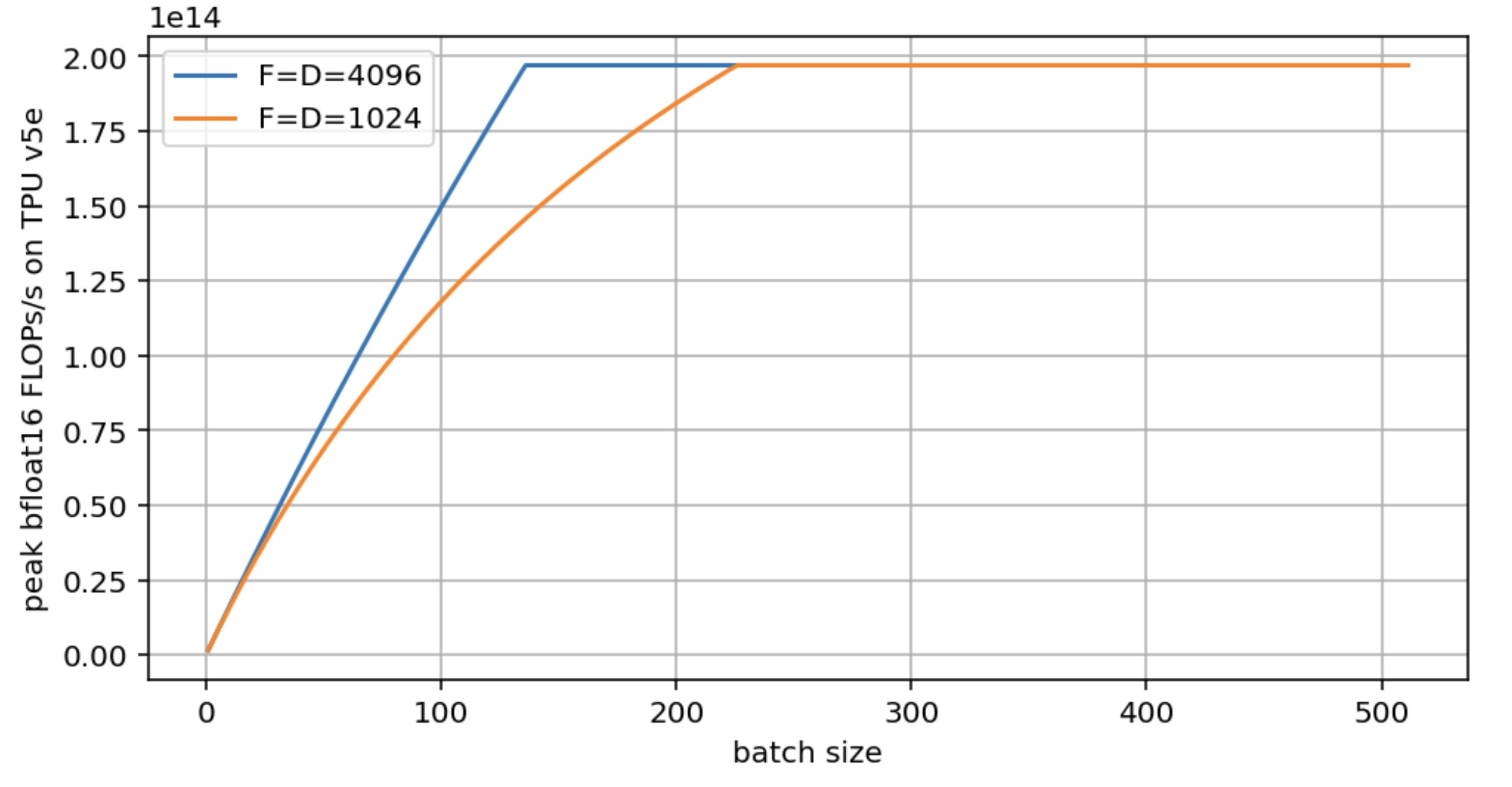
Source: JAX Scaling Book, “All About Rooflines”, MIT License. The original exercise compares roofline throughput for different matrix sizes as batch size increases.

7. Quantization을 Roofline으로 보기

Quantization은 roofline에서 두 가지를 바꾼다.

1. 이동해야 하는 bytes를 줄인다.
2. hardware가 low precision compute를 지원하면 peak OPs/s도 바꾼다.

예를 들어 BF16 matmul에서 INT8 weight-only로 바꾼다고 하자.

bf16 activation: 2BD bytes
int8 weight: DF bytes
bf16 output: 2BF bytes

작은 B에서는 weight read DF가 지배적이므로, weight bytes가 절반으로 줄면 arithmetic intensity가 올라간다. 그래서 compute-bound로 넘어가는 critical batch size가 낮아질 수 있다.

하지만 INT8 compute를 native로 쓰면 peak OPs/s도 올라간다. 이 경우 hardware critical intensity도 같이 올라간다. 그래서 “bytes가 줄었으니 무조건 compute-bound로 간다”는 식으로 단순화하면 안 된다.

Week 4의 실험 결론도 같은 방향이다.

Case	Roofline interpretation
AWQ INT4 fused kernel이 빨라짐	bytes 감소가 실제 kernel path에서 latency 감소로 이어짐
bitsandbytes NF4가 느려짐	bytes 감소보다 dequant/kernel overhead가 큼
Orin INT4 projection	edge bandwidth-bound regime에서는 bytes 감소가 직접 이득

8. Network Communication Roofline

Roofline은 HBM에만 쓰는 모델이 아니다. Accelerator 사이 통신에도 그대로 적용된다.

예를 들어 matrix multiplication을 두 chip에 나눴다고 하자. 각 chip은 compute를 절반만 하지만, partial result를 서로 보내고 합쳐야 한다.

이때 비교해야 하는 것은:

T_math = local FLOPs / local FLOPs/s
T_comms = bytes sent across interconnect / interconnect bandwidth

단일 GPU에서는 HBM roofline을 보지만, tensor parallelism에서는 NVLink/ICI/InfiniBand roofline을 봐야 한다.

Parallelism	Dominant roofline
Tensor parallelism inside node	NVLink / NVSwitch collective roofline
TPU sharding inside slice	ICI roofline
Pipeline parallelism across nodes	activation transfer roofline
Expert parallelism	AllToAll network roofline
Data parallelism training	gradient AllReduce roofline

이 관점은 DSA 글의 ops:comms ratio와 같은 이야기다.

ops:comms ratio = compute throughput / communication bandwidth

9. Roofline을 Inference에 적용하는 순서

실제 inference 시스템을 볼 때는 다음 순서로 계산한다.

1. Workload phase를 나눈다: prefill, decode, batched decode, verification.
2. 각 phase의 주요 kernel을 찾는다: GEMM, GEMV, attention, sampling, collective.
3. FLOPs를 대략 계산한다.
4. 이동 bytes를 계산한다: weights, activations, KV cache, network tensor.
5. Arithmetic intensity를 구한다.
6. Hardware critical intensity와 비교한다.
7. Profile로 overhead와 overlap 실패를 확인한다.

간단한 decision table은 다음과 같다.

Observation	Likely next step
Low intensity, high HBM traffic	quantization, fusion, better layout
High intensity, low Tensor Core utilization	tiling, batch size, kernel choice
Collective time dominates	sharding strategy or topology change
Capacity-bound	quantization, sharding, KV cache compression
GPU-Util high but FLOPs low	profiler로 SM throughput/HBM throughput 확인

10. 이 레포와의 연결

Repository topic	Roofline connection
Week 1 performance metrics	throughput, latency, utilization을 upper/lower bound로 해석한다.
Week 2 hardware foundations	GEMM/GEMV roofline plot을 직접 측정한다.
Week 3 KV cache	decode attention의 bytes/token을 계산한다.
Week 4 quantization	bytes 감소가 latency 감소로 이어지는 조건을 설명한다.
DSA appendix	memory movement와 ops:comms 설계 원칙의 수학적 기반이다.
GPU/TPU appendix	hardware critical intensity를 GPU/TPU별로 비교한다.

11. Practical Tips and Notes

Roofline은 정확한 예측기가 아니라 빠른 필터다

Roofline은 10초 안에 “이 주장이 말이 되는가”를 판단하게 해준다. 하지만 정확한 latency를 예측하려면 다음을 더 봐야 한다.

Missing factor	Example
Kernel launch overhead	small batch decode
Memory latency	bandwidth가 충분해도 random access가 느림
Cache hit rate	L2/SMEM reuse
Dequant overhead	low-bit inference
Scheduler overhead	serving batch packing
Collective latency	small message AllReduce
Overlap failure	compute와 communication이 따로 직렬화됨

따라서 roofline은 “profiling을 대체하는 도구”가 아니라 “profiling을 어디서 시작할지 정하는 도구”다.

x축은 log scale로 보는 경우가 많다

원문 roofline plot은 보통 log-log로 그린다. Arithmetic intensity와 throughput이 몇 자릿수씩 차이 나기 때문이다. 이 노트의 SVG는 개념 설명을 위해 단순 선형 그림처럼 그렸지만, 실제 분석에서는 log scale이 더 유용하다.

Memory-bound가 항상 나쁜 것은 아니다

Decode는 본질적으로 memory-bound일 수 있다. 이때 목표는 compute-bound로 억지로 바꾸는 것이 아니라, memory-bound regime에서 bytes/token과 overhead를 줄이는 것이다.

예를 들어:

Technique	What it reduces
W4A16 quantization	weight bytes
GQA/MQA/MLA	KV cache bytes
PagedAttention	fragmentation and allocation waste
FlashAttention	attention intermediate HBM traffic
Kernel fusion	intermediate tensor round-trips

12. Check Questions

1. T_math와 T_comms는 각각 무엇을 의미하는가?
2. 왜 runtime lower bound를 max(T_math, T_comms)로 볼 수 있는가?
3. Arithmetic intensity가 낮으면 어떤 bound에 걸리기 쉬운가?
4. Dot product의 arithmetic intensity가 낮은 이유는 무엇인가?
5. Transformer matmul에서 intensity가 대략 local token batch B가 되는 이유는 무엇인가?
6. H100 BF16 matmul의 critical batch size가 대략 300이라는 말은 무엇을 뜻하는가?
7. Quantization은 roofline의 어느 부분을 바꾸는가?
8. Tensor parallelism에서는 왜 HBM roofline 대신 interconnect roofline을 봐야 하는가?
9. Roofline으로 설명되지 않는 overhead에는 무엇이 있는가?
10. Week 2의 GEMV/GEMM 전환을 roofline 관점으로 설명해보라.